On the road to machine learning, we will find that the basic algorithms are inseparable from the knowledge of mathematical statistics. This blog is to assist you to better understand Confidence Interval and Confidence Level from fundamental concepts to practical instances.

---

Blog Navigation

• • 1 Fundamental definition and feature.
  • 1.1 T-test (T-distribution).
    • 1.1.1 Definition of T-test.
    • 1.1.2 Feature of T-test.
  • 1.2 Confidence Interval and Confidence Level.
  • 1.2.1 Definition of Confidence Interval.
  • 1.2.2 Definition of Confidence Level.
  • 1.2.3 Confidence Level from a region perspective.
  • 1.2.4 Feature of Confidence Level.
• • 2 Practical Instantiation.
  • 2.1 Background Description.
  • 2.2 Problem Solving.
  • 2.2.1 Formula Manipulation.
  • 2.2.2 T-Table Look-Up
  • 2.2.3 Obtain Confidence Interval.
• • 3 End.

---

1 Fundamental definition and feature.

1.1 T-test (T-distribution).

1.1.1 Definition of T-test.

In general,T-test can be classified as three tests: Single Population Test, Double Population Test, and Paired Sample Test.Without doubt, T-test is closely related to the T-distribution.To simplify our problem, we only consider Single Population Test here as our topic.

A Single Population T-test tests whether a sample mean differs significantly from a known population mean. When the population distribution is normal, such as the population standard deviation is unknown and the sample size is less than 30, then the deviation statistic between the sample mean and the population mean is T-distributed.In other word, the purpose of T-test is to determine whether the mean difference between two types of samples on a certain variable is significant, which is also the reason why we constructing T-test.

The formula of Single Population T-test is:

$$t = \frac{\overline{X} - \mu_{0}}{\frac{\sigma_{x}}{\sqrt{N}}}$$

Here, \(\overline{X}\) represents sample mean, \(\mu_{0}\) represents population mean, \(\sigma_{x}\) represents standard deviation and N represents the number of samples.In Single Population T-test, the degree of freedom \(df = N - 1\). With more professional terminology, \(\frac{\sigma_{x}}{\sqrt{N}}\) stands for Standard Error of Mean, which is:

$$SEM = \frac{\sigma_{x}}{\sqrt{N}}$$

SEM is a quite significant concept.Instead of the standard deviation of the population, SEM utilizes the sample standard deviation.In light of above, we can conclude that the t-value can be interpreted as the extent to which the sampling mean deviates from the population mean correspond to the SEM.

1.1.2 Feature of T-test.

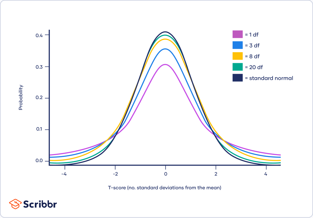
[figure source: www.scribbr.co.uk]

As the figure above, we can observe that when the degree of freedom increments, the curve becomes narrower and taller, and more resemble as normal distribution.Conversely, it becomes flatter.In the matter of fact, when \(df \geq 30\), the T-distribution curve and the normal distribution curve are difficult to distinguish with the naked eyes.

1.2 Confidence Interval and Confidence Level.

1.2.1 Definition of Confidence Interval.

All confidence intervals are based on the concept of point estimation, in which a single sample is taken from the population and its sample mean is used as a point estimate of the population mean.The confidence interval is where we add a floating range to the point estimate, and the value within this interval is acceptable to the forecast.

Since the mean of the point estimate is easy to find, what we really need to determine is the upper and lower boundaries(critical points) of confidence interval, that is, the floating range.We will elaborate it detailedly in the following content.

1.2.2 Definition of Confidence Level.

To better understand the confidence level, we need to introduce Significance Level \(\alpha\) firstly.By definition, Significance level refers to the probability that the null hypothesis is wrongly rejected when the null hypothesis itself is true in a statistical hypothesis test.Significance Level is usually considered a prescribed two-sided threshold, i.e. one side is \(\alpha/2\).Common values of \(\alpha\) are 0.05, 0.01, and so on.

Confidence Level is an abstraction of Confidence Interval.By repeatedly building the confidence interval, we obtain a set of confidence intervals.The confidence level is the frequency of the confidence interval that contains the real population mean in the set over the number of confidence intervals in the set.However,this formula is inefficient.In contrary,there exists a more efficient formula:

$$ConfidenceLevel = 1 - \alpha$$

1.2.3 Confidence Level from a region perspective.

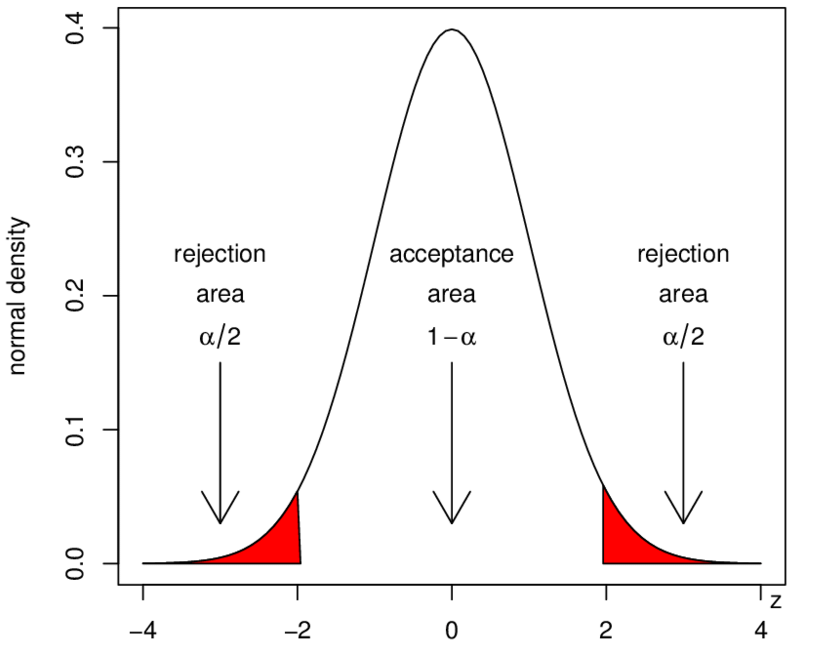
Let \(\mu_{real}\) represents the population sample mean.Assuming we have the floating range by some means (I will discuss it later), we add or subtract the floating range from both sides with \(\mu_{real}\) as the center to get a closed interval, we call this closed interval as Acceptance Region, and the remaining unclosed interval as Reject Region.

However, since the floating range is fixed, then the confidence interval we construct for each point estimate and the acceptance region have the same width. Therefore, we can conclude that:
• If \(\mu_{sample}\) falls in acceptance region, then thesample confidence interval constructed by \(\mu_{sample}\) must contain \(\mu_{real}\).
• If \(\mu_{sample}\) falls on reject region, then the sample confidence interval constructed by \(\mu_{sample}\) must not contain \(\mu_{real}\).

In light of above, from the perspective of region, a confidence level of \((1 - \alpha)\) is equivalent to a sampling distribution acceptance area of \((1 - \alpha)\).

1.2.4 Feature of Confidence Level.

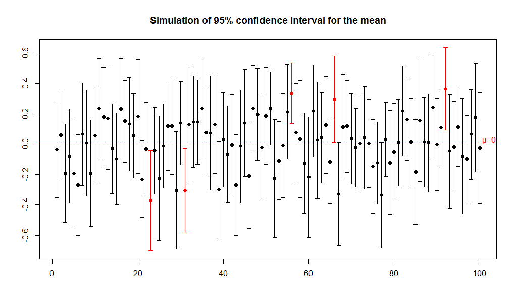
Common confidence levels include 90%, 95%, and 99%.It’s worth noting that if we take the 95% confidence level as an instance, the 95% does not represent that there exists a 95% probability for \(\mu_{real}\) to fall within the confidence interval constructed by \(\mu_{sample}\).Instead, it represents that the confidence interval with a large number of repeated build point estimates has a 95% probability of containing \(\mu_{real}\).

Here are two significant features for Confidence Level:
▸ When the confidence level is unchanged, the larger the sample size, the narrower the confidence interval.
▸ When the sample size is unchanged, the higher the confidence level, the wider the confidence interval.

---

2 Practical Instantiation.

2.1 Background Description.

Suppose we have an analytical population with unknown population mean \(\mu_{real}\).Assuming that our confidence interval is set to be \(\alpha\) and \(\sigma_{x}\) is the standard deviation of our population.Our goal is to obtain the confidence interval of the analytical population by sampling the sample with size \(N\)(which is point estimation).Now, presuming that the mean of our point estimation is \(\mu_{s}\).

2.2 Problem Solving.

2.2.1 Formula Manipulation.

Since the distribution of our multiple samples conforms to the T-distribution, our critical \(\overline{X}\) value needs to be calculated by the T-value. Recall that the formula of t-value is:

$$t_{bound} = \frac{\overline{X}_{bound} - \mu_{s}}{\frac{\sigma_{x}}{\sqrt{N}}}$$

There is no need to wonder why \(\mu_{s}\) displaces the population mean \(\mu_{0}\) here, because point estimation utilizes the sample mean to estimate the population mean, and that is:

$$\widehat{\mu_{0}} = \mu_{s}$$

Now, we transform the formula for t-value into another form:

$$\overline{X}_{bound} = \mu_{s} + t_{bound} \cdot \frac{\sigma_{x}}{\sqrt{N}}$$

The only term left undetermined by the quation is the value of \(t_{bound}\).

2.2.2 T-Table Look-Up

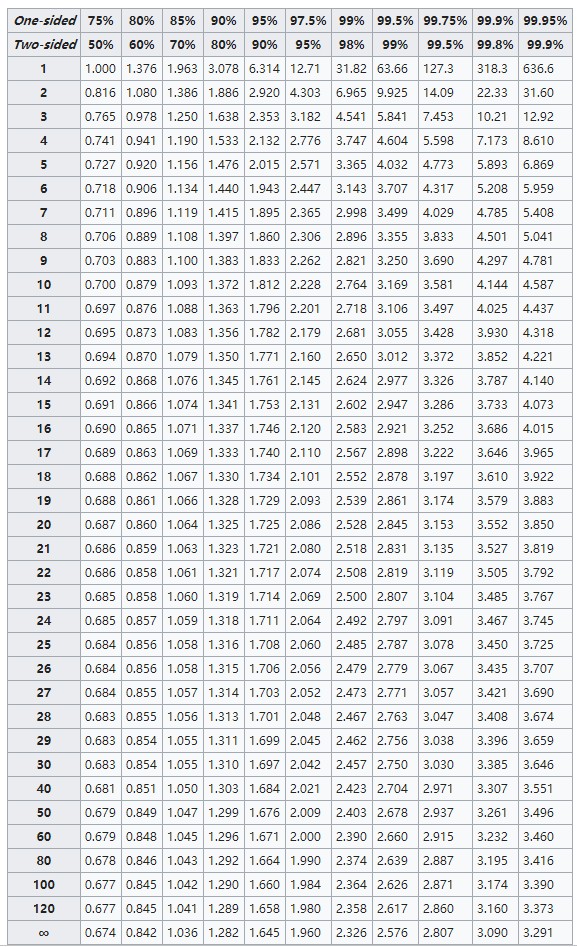
This T-Table shows the range of the corresponding rejection region(first two rows) and the values of the corresponding degrees of freedom(first column). Recall that the formula for degree of freedom and TwoSide probability is:

$$ \begin{equation} \begin{cases} df = N - 1 \\ TwoSide = 1 - \alpha \end{cases} \end{equation} $$

Depending on the confidence level and the degree of freedom, we lock the t-value in the table.

It is quite significant to be careful here that the t-values in our table are all positive, but in fact there is a t-value of the same absolute magnitude in the negative half axis for the two-sides t:

$$t_{bound} = \pm value$$

2.2.3 Obtain Confidence Interval.

After getting two values of \(t_{bound}\), we can obtain two values of \(\overline{X}_{bound}\), which are critical points.The smaller value is for the lower boundary of confidence interval, and the larger value is for the upper boundary of confidence interval.Definitely, we obtain the confidence interval for \(\mu_{s}\):

$$[\mu_{s} - |t_{bound}| \cdot \frac{\sigma_{x}}{\sqrt{N}} , \mu_{s} + |t_{bound}| \cdot \frac{\sigma_{x}}{\sqrt{N}}]$$

As you may have noticed, the so-called floating range is actually \(2 \cdot |t_{bound}| \cdot \frac{\sigma_{x}}{\sqrt{N}}\). This is also the width of acceptance region.

---

3 End.

We’ve ultimately got the confidence intervals we want, and I’m sure you know the concepts inside out! Note again: The confidence interval we construct does not contain \(\mu_{real}\) with the probability of \(\alpha\), but from the perspective of macroscopic multiple point estimates, the confidence intervals of \(\alpha\) percent contain \(\mu_{real}\).

Thank you for reading my blog, if you like my blog, please offer me a comment to support!